(Dave Case, January 2005)
The sander program has a fairly powerful capability of estimating the free energy for a transformation between two different potential functions. I'm assuming that you have read the appropriate sections of the Users' Manual. Here I disucss an example calculation, trying to see if I can reproduce some literature values.
I am looking at the transformation toluene -> nothing in water (analogue of the phe side chain), as reported by M.R. Shirts, J.W. Pitera, W.C. Swope and V.S. Pande, "Extremely precise free energy calculations of amino acid side chain analogs: Comparison of common molecular mechanics force fields for proteins", J. Chem. Phys. 119, 5740-5761 (2003).
We are basically trying to reproduce here the force field and numbers for the "phe" entry in the Amber portion of Table 1 of this paper. However, this is not an attempt at an *exact* reproduction (which would require lots of things Amber can't do), but to get the closest we can within the Amber codes. In particular, we are getting the density of the system from MD runs using PME and a long-range van der Waals correction, not with the cutoff simulations reported in this paper. But aside from this difference, things should be pretty directly comparable.
Following Shirts et al., we consider two separate free energy transformations, one where the charges on toluene are removed, and a second where the LJ interactions between tolune and water are morphed to zero. The first is a much simpler calculation than the second.
There are of course a variety of ways to carry out these simulations. The Coulomb part can use linear mixing TI (klambda=1), with just a few samples for lambda. Don't forget that you need to carry out a parallel vacuum simulation, and subtract the two results. The vacuum calculations converge really fast, since there are almost no degrees of freedom to average over (toluene is a very rigid molecule).
The vdw part is harder to converge. My current thinking is that the best results come with klambda=6, but you can get nearly as good results with klambda = 4 or 5, as shown below. Of course, this is all a matter of efficiency: you should get the same results with long enough sampling regardless of the value of klambda.
Note: This is a fairly "advanced" tutorial: you should only try free energy simulations after you are comfortable equilibrating and running more conventional jobs that are covered in other tutorials. For this reason, I am skipping some of the details (exactly how to equilibrate things, for example), in order to concentrate on those features that are unique to free energy calculations. I am also assuming that you are familiar with the basic theory of thermodynamic intergration calculations; if not, I suggest Tom Simonson's article "Free energy calculations", in Computational Biochemistry and Biophysics, edited by Becker, Mackerell, Roux and Watanabe, (New York: Marcel Dekker, 2001), pp. 169-197. The Shirts paper cited above is then a nice place to see some of the advanced considerations that go into carrying out this sort of simulation.
The model used by Michael Shirts for a phenyalanine side chain is toluene, and I followed his prescription for assigning the charges and other parameters. I used LEaP to set up two files for toluene that have the beginning and endpoints of these transformations.
First, I entered xleap and edited the PHE residue to remove the backbone and create toluene, so that my structure looks like this:
Next, I selected all the atoms, and used the menu item "Edit Selection". This brings up a spreadsheet like the one shown below, and I filled in all of the entries as shown. Note that the "Delta charge" for each atom is the opposite of its "normal" charge, so that all that atoms in the perturbed state have zero charge.

I then exited the table and issued the commands:
	saveOff PHE phe_coul.off
	saveAmberParmPert PHE prmtop.coul.vac prmcrd.coul.vac
The files are now ready to run a charging free energy in vacuum, which you need to do to compare to the solvated calculation to come later. Here is an example of an input file for sander:
	  neutralize toluene
	 &cntrl
	   ntr=0,
	   nstlim =100000, nscm=2000, ntave=10000,
	   ntx=5, irest=1, ntb=0, ntpr=200,
	   dt=0.001, nrespa=2,
	   ntt=1, temp0 = 300., tautp=2.0,
	   ntc=2, ntf=2, tol=0.000001,
	   ntwr = 10000, ntwx=0,
	   icfe=1, clambda=0.5,
	 /
Note that I am setting clambda to 0.5 here; you could try other values, but the results won't change hardly at all, since there is no "environment" to respond to changes in charges. Running this converges quickly to give me an average value of <dV/dl> of -0.46 kcal/mol. Here is a little bit of my output file:
			  -------------------------------------------------------
			  Amber 7  SANDER                   Scripps/UCSF 2002
			  -------------------------------------------------------

	|      Fri Oct 18 08:21:20 2002

	  [-O]verwriting output

	File Assignments:
	|  MDIN: mdin
	| MDOUT: eq2.o
	|INPCRD: eq1.x
	|  PARM: prmtop.coul.vac
	|RESTRT: eq2.x
	|  REFC: refc
	| MDVEL: mdvel
	|  MDEN: mden
	| MDCRD: mdcrd
	|MDINFO: mdinfo
	|INPDIP: inpdip
	|RSTDIP: rstdip


	 Here is the input file:

	  neutralize toluene
	 &cntrl
	   ntr=0,
	   nstlim =100000, nscm=2000, ntave=10000,
	   ntx=5, irest=1, ntb=0, ntpr=200,
	   ntp=0, taup=2.0,
	   dt=0.001, nrespa=2,
	   ntt=1, temp0 = 300., tautp=2.0,
	   ntc=2, ntf=2, tol=0.000001,
	   ntwr = 10000, ntwx=0,
	   icfe=1, clambda=0.5,
	 &end

	 ....

	Running a free energy calculation with lambda =  0.500

	 ....

	 NSTEP =    200 TIME(PS) =    10.200  TEMP(K) =   296.02  PRESS =     0.0
	 Etot   =      26.7094  EKtot   =      11.4709  EPtot      =      15.2384
	 BOND   =       6.2906  ANGLE   =       5.1183  DIHED      =       0.0722
	 1-4 NB =       3.9324  1-4 EEL =      -0.5576  VDWAALS    =      -0.3797
	 EELEC  =       0.7622  EHBOND  =       0.0000  RESTRAINT  =       0.0000
	 DV/DL  =      -0.4093
	 ------------------------------------------------------------------------------

	 .....

	|===============================================================================

		  A V E R A G E S   O V E R   50000 S T E P S


	 NSTEP = 100000 TIME(PS) =   110.000  TEMP(K) =   304.59  PRESS =     0.0
	 Etot   =      27.1592  EKtot   =      11.8028  EPtot      =      15.3565
	 BOND   =       4.9797  ANGLE   =       4.2533  DIHED      =       2.3002
	 1-4 NB =       3.8807  1-4 EEL =      -0.5570  VDWAALS    =      -0.2896
	 EELEC  =       0.7893  EHBOND  =       0.0000  RESTRAINT  =       0.0000
	 DV/DL  =      -0.4646
	 ------------------------------------------------------------------------------


		  R M S  F L U C T U A T I O N S


	 NSTEP = 100000 TIME(PS) =   110.000  TEMP(K) =    47.64  PRESS =     0.0
	 Etot   =       0.2891  EKtot   =       1.8461  EPtot      =       1.9234
	 BOND   =       1.6496  ANGLE   =       1.3617  DIHED      =       1.2634
	 1-4 NB =       0.4003  1-4 EEL =       0.0601  VDWAALS    =       0.0938
	 EELEC  =       0.0281  EHBOND  =       0.0000  RESTRAINT  =       0.0000
	 DV/DL  =       0.0807
	 ------------------------------------------------------------------------------


		  DV/DL, AVERAGES OVER   50000 STEPS


	 NSTEP = 100000 TIME(PS) =   110.000  TEMP(K) =     0.00  PRESS =     0.0
	 Etot   =       0.0000  EKtot   =       0.0000  EPtot      =      -0.4646
	 BOND   =       0.0000  ANGLE   =       0.0000  DIHED      =       0.0000
	 1-4 NB =       0.0000  1-4 EEL =       1.1140  VDWAALS    =       0.0000
	 EELEC  =      -1.5786  EHBOND  =       0.0000  RESTRAINT  =       0.0000
[sample-rms]*sqrt[correlation-time/length-of-simulation]
where correlation-time/length-of-simulation is an estimate of the number of "independent samples" that have been accumulated. In our case, the correlation-time is quite short (probably below 0.1 psec), since on fast vibrational motions are influencing the result. Hence, the expected error in the mean is about 0.081 * sqrt[ 0.1/50 ] = 0.004 kcal/mol.
We are now ready to run the corresponding simulation in water. We can use the off file we created above to get things going, giving the following commands to LEaP:
	source leaprc.ff94
	loadOff phe_coul.off
	solvateOct PHE TIP3PBOX 12.0 0.8
	saveAmberParmPert PHE prmtop.coul.wat prmcrd.coul.wat
We would then equilibrate this system in the usual way. This time, we need to use more than one value of clambda, since the water environment around the solute will depend upon its charges. I used a perl script to automate this procedure:
	#! /usr/bin/perl -w

	@clambda=( 0.11270, 0.5, 0.88729 );

	foreach $in ( 0 .. 2 ){

		$out = $in + 1;

		#    equilibration:

		open( MDIN, ">mdin");
		print MDIN <<EOF;
		  neutralize toluene
		 &cntrl
		   ntr=0,
		   nstlim =20000, nscm=2000, ntave=5000,
		   ntx=1, irest=0, ntb=2, ntpr=100, tempi=300.0, ig=974651,
		   ntp=1, taup=1.0,
		   dt=0.001, nrespa=1,
		   ntt=1, temp0 = 300., tautp=2.0,
		   ntc=2, ntf=2, tol=0.000001,
		   ntwr = 10000, ntwx=0,
		   icfe=1, clambda=${clambda[$in]},
		   cut=9.0,
		 /
		EOF
		close MDIN;

		system("sander -O -i mdin -p prmtop.vdw -c eq$in.x -o eq$out.oe -r eq$out.xe" );

		#    production:

		open( MDIN, ">mdin");
		print MDIN <<EOF;
		  neutralize toluene
		 &cntrl
		   ntr=0,
		   nstlim =100000, nscm=2000, ntave=5000,
		   ntx=7, irest=1, ntb=1, ntpr=100,
		   ntp=0, taup=2.0,
		   dt=0.001, nrespa=2,
		   ntt=0, temp0 = 300., tautp=2.0,
		   ntc=2, ntf=2, tol=0.000001,
		   ntwr = 10000, ntwx=0,
		   icfe=1, clambda=${clambda[$in]},
		   cut=9.0,
		 /
		EOF
		close MDIN;

		system("sander -O -i mdin -p prmtop.vdw -c eq$out.xe -o eq$out.o -r eq$out.x" );

	}
For each value of clambda, this sets up a constant pressure equilibration run, followed by a constant energy production run. Obviously, the length of these runs (and other parameters) would need to be adjusted for the situation. Water relaxes quickly around this small, almost rigid solute, so 20 psec of equilibration and 100 psec of production should be sufficient. For proteins, the required times might be longer. It's easy enough to run longer simulations to see what happens.
I have also used only three values of clambda, based on experience that charging free energies are very smooth funcitons of clambda. Again, this is something that you should check for yourself.
      at lambda = 0.11270, <dV/dl> = 4.13 +/- 2.26

      at lambda = 0.5    , <dV/dl> = 1.52 +/- 1.80

      at lambda = 0.88729, <dV/dl> =-0.26 +/- 1.49
Three-point Gaussian integration of the above yields 1.75 kcal/mol.
The "vacuum" results gave -0.46 kcal/mol.
The water - vaccum difference is thus 2.18 kcal/mol
This can be compared to the Shirts et al. value of 2.35 kcal/mol.
Our uncertainty is probably about +/- 0.2 kcal/mol.
Now that we have removed all charges from the system, we are in a position to change all of the atoms in the molecule to dummy atoms, that is, to make the whole molecule disappear. Again we have to do this both in vacuum and in water.
To set up the system, I again used xLEaP to edit the parameters of my residue, so that it looks like this:
I made two types of dummy carbons (one for the methyl carbon, and one for the aromatic ring), and two corresponding types of dummy hydrogens. The parameters for these dummy atoms are the same as for the real atoms, except that the van der Waals parameters are set to zero. This can be done using a frcmod file:
	  convert toluene to nothing
	MASS
	DH   1.008
	DI   1.008
	DC   12.01
	DD   12.01

	BOND
	DC-DH  367.0    1.080
	DC-DC  469.0    1.400
	DC-DD  317.0    1.510
	DD-DI  340.0    1.090

	ANGL
	DC-DC-DH    35.0      120.00
	DC-DC-DC    63.0      120.00
	DC-DC-DD    70.0      120.00
	DC-DD-DI    50.0      109.50
	DI-DD-DI    35.0      109.50

	DIHE
	X -DC-DC-X    4   14.50        180.0             2.
	X -DC-DD-X    6    0.00          0.0             2.

	IMPR
	X -X -DC-DH         1.1          180.          2.
	DC-DC-DC-DD         1.1          180.          2.

	NONB
	  DH          1.0000  0.000
	  DI          1.0000  0.000
	  DC          1.0000  0.000
	  DD          1.0000  0.000
Now the procedure is really very similar to that for the charging free enegies, but with some changes. First, since atoms are disappearing, you need to set klambda to be a larger value; results for 4,5, and 6 are shown below. Second, you need many more intermediate lambda values, since the <dV/dl> vs. lambda curve is much less smooth.
I used ten values of clambda from 0.05, 0.15, ...0.85, and additional values at 0.90, 0.92, 0.94, 0.96 and 0.98. Here are the results, with estimate uncertainties shown as well:
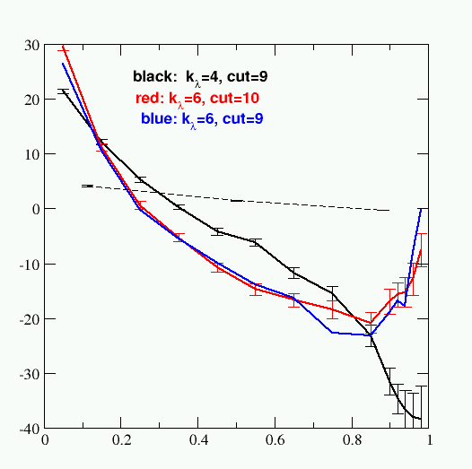
The charging free energy results are shown as the dashed line. Note that the error bars and complexity of the vdW curves are much greater than those for the charging free energy. Removing the charges is an "easy" free energy change, whereas making everything disappear is a "difficult" transformation.
For the klambda = 6 values, I used the trapezoidal rule to estimate the integral. Summing everything together gives a total of -6.44 kcal/mol. The "vacuum" part was quickly evaluated to be -3.74 kcal/mol. Hence, water - vacuum is -2.70 kcal/mol, compared to the Shirts et al. result of -2.45 kcal/mol (including the long-range vdW correction, which is automatically included in Amber). Again, the results agree to within about 0.2 kcal/mol. I could do longer sampling to see if things change, but you must also remember that Michael Shirts used a cutoff simulation (which is not available in sander) to get the densities for his calculations, whereas we are using the densities that come from an Ewald simulation. So there will inevitably be minor differences in the final results.
Note that the electrostatic and van der Waals contributions nearly cancel each other: it costs energy to remove the charges; even though they are small, they have a little bit of favorable interaction energy with the water dipoles. But you gain energy by removing the uncharged, "oily" tolune from water; this is like the unfavorable (hydrophobic) interaction of completely nonpolar solutes with water.
Also note that the assignment of part of the free energy change to "electrostatics" and part to "van der Waals" is not unique. If I had chosen a different path, the contributions of these two terms could change, although the total free energy for the complete process should be the same. Even though there is not a unique decomposition into electrostatic and van der Waals terms, the decomposition used here is often qualitatively helpful in understanding free energy changes.
Running free energy simulations in sander is not fundamentally difficult, but you do have to pay careful attention to setting up the system parameters, and in looking at the output to be sure it makes sense. There is no automated procedure to prepare the parameter files to morph one type of group into another. You will have to make choices, and explore for yourself the consequences of various alternatives.
The ideas shown here could also be used to convert one functional group into another, (rather than converting everything to dummy atoms). Always remember that you need to carry out two sides of some thermodynamic cycle, and subtract the two results. The "absolute" energy along any one cycle is almost never meaningful by itself.
Another type of free enegy calculation looks at conformational changes, rather than the "alchemical" changes discussed here. To look at those in sander, you will want to to at the umbrella sampling section of the Users' Manual, and would not use the techniques outlined here.