(Note: These tutorials are meant to provide illustrative examples of how to use the AMBER software suite to carry out simulations that can be run on a simple workstation in a reasonable period of time. They do not necessarily provide the optimal choice of parameters or methods for the particular application area.)
Copyright Ross Walker 2004

TUTORIAL 6 - AMBER 8 VERSION - SECTION 2

A Coupled Potential QMMM Simulation

By Ross Walker

PLEASE NOTE THIS TUTORIAL IS FOR AMBER 8 ONLY.
AN AMBER 9 QM/MM TUTORIAL IS AVAILABLE HERE

2) Classical MD

Now we have our topology and coordinate files we are ready to carry out classical molecular dynamics. First things first though we need to minimise our system to remove any bad contacts created by solvation and also to allow our artificially created NMA structure to relax. For this we will run 500 steps of minimisation. Our input file is very similar to files we have used in the previous tutorials. We are not using periodic boundaries so we have NTB=0. We will also not use SHAKE (NTC=1 - the default) and since we have a solvent cap which we don't want to boil off into space we will add a weak restraint force of 1.5 KCal/mol/Angstrom (FCAP=1.5). We do not explicitly need to tell sander that a solvent cap is present since it will ascertain this from the prmtop file. Here is our input file:

Once we have minimised the system we will run 1,000fs of molecular dynamics at a constant temperature of 300K. Normally we would slowly heat our system to 300K but since this is just a small NMA molecule in solution it should be fairly stable and should survive being started out at 300K. During the MD we will write to both our output file and mdcrd file every step. In this way we will be able to see the detailed motion of our system. At the expense of slowing the simulation down while it writes a considerable amount of information to disk. Here is the input file for the MD run:

Now we run the minimisation and md. Feel free to script the run if you want so it runs the minimisation and then automatically runs the MD. In this way you can go off and enjoy a nice cup of coffee while it runs.

$AMBERHOME/exe/sander -O -i min_classical.in -o min_classical.out -p NMA.prmtop -c NMA.inpcrd -r NMA_min_classical.crd

$AMBERHOME/exe/sander -O -i md_classical.in -o md_classical.out -p NMA.prmtop -c NMA_min_classical.crd -r NMA_md_classical.rst -x NMA_md_classical.mdcrd

This should take about 3 mins to run. Here are the output files: min_classical.out, NMA_min_classical.crd, md_classical.out, NMA_md_classical.mdcrd

Now, let's do two things. First of all we will visualise our MD trajectory in VMD and secondly we will use ptraj to create an average structure for us.

Step 1 - VMD. Fire up VMD and load the NMA topology file (remember to select parm7) and then load the NMA_md_classical.mdcrd file into this molecule. Remember, we have not used periodic boundaries here so select "crd" (not "crdbox").

While it is good to see our big cap of water "floating" about we are more interested in the dynamics of the NMA residue so let's remove the water.

Graphics->Representations
In Selected Atoms type:
all not water
And hit apply
At the same time change the drawing method to CPK.

You should now be able to watch a movie of our NMA molecule "wiggling" about.

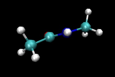
The thing to notice is how planar the amide C-N-H group remains during the simulation. This is largely artificial since the nitrogen atom has a lone pair which acts to force the hydrogen out of plane. This is a deficiency of the classical force field as it is currently implemented. Work is under way to try to improve this.

Step 2 - PTRAJ. To create an average structure from our classical md simulation we will use ptraj. Ptraj is a very powerful analysis program that comes with AMBER 8. It can do a huge range of manipulations and calculations on amber and charmm trajectory files. See the AMBER manual for more details. Here we will simply get it to write us the average structure from the 1,000 structures written during our 1 ps of MD. Here is the input file for ptraj:

trajin NMA_md_classical.mdcrd
average NMA_md_classical_average.pdb pdb

Run ptraj as follows:

$AMBERHOME/exe/ptraj NMA.prmtop < ave_classical.ptraj

Here's the average structure: NMA_md_classical_average.pdb. If you want take a look at it in VMD.